A blog on statistics, methods, philosophy of science, and open science. Understanding 20% of statistics will improve 80% of your inferences.

Tuesday, March 14, 2017

Equivalence testing in jamovi


One of the challenges of trying to get people to improve their statistical inferences is access to good software. After 32 years, SPSS still does not give a Cohen’s d effect size when researchers perform a t-test. I’m a big fan of R nowadays, but I still remember when it I thought R looked so complex I was convinced I was not smart enough to learn how to use it. And therefore, I’ve always tried to make statistics accessible to a larger, non-R using audience. I know there is a need for this – my paper on effect sizes from 2013 will reach 600 citations this week, and the spreadsheet that comes with the article is a big part of its success.

So when I wrote an article about thebenefits of equivalence testing for psychologists, I also made a spreadsheet. But really, what we want is easy to use software that combines all the ways in which you can improve your inferences. And in recent years, we see some great SPSS alternatives that try to do just that, such as PSPP, JASP, and more recently, jamovi.

Jamovi is made by developers who used to work on JASP, and you’ll see JASP and jamovi look and feel very similar. I’d recommend downloading and installing both these excellent free software packages. Where JASP aims to provide Bayesian statistical methods in an accessible and user-friendly way (and you can do all sorts of Bayesian analyses in JASP), the core aim of jamovi is wanting to make software that is ‘“community driven”, where anyone can develop and publish analyses, and make them available to a wide audience’. This means that if I develop statistical analyses, such as equivalence tests, I can make these available through jamovi for anyone who wants to use these tests. I think that’s really cool, and I’m super excited my equivalence testing package TOSTER is now available as a jamovi module. 

You can download the latest version of jamovi here. The latest version at the time of writing is 0.7.0.2. Install, and open the software. Then, install the TOSTER module. Click the + module button:


Install the TOSTER module:


And you should see a new menu option in the task bar, called TOSTER:


To play around with some real data, let’s download the data from Study 7 from Yap et al, in press, from the Open Science Framework: https://osf.io/pzqj2/. This study examines the effect of weather (good vs bad days) on mood and life satisfaction. Like any researcher who takes science seriously, Yap, Wortman, Anusic, Baker, Scherer, Donnellan, and Lucas made their data available with the publication. After downloading the data, we need to replace the missing values indicated with NA with “” in a text editor (CTRL H, find and replace), and then we can read in the data in jamovi. If you want to follow along, you can also directly download the jamovi file here.

Then, we can just click the TOSTER menu, select a TOST independent samples t-test, select ‘condition’ as condition, and analyze for example the ‘lifeSat2’ variable, or life satisfaction. Then we need to select an equivalence bound. For this DV we have data from approximately 117 people on good days, and 167 people on bad days. We need 136 participants in each condition to have 90% power to reject effects of d = 0.4 or larger, so let’s select d = 0.4 as an equivalence bound. I’m not saying smaller effects are not practically relevant – they might very well be. But if the authors were interested in smaller effects, they would have collected more data. So I’m assuming here the authors thought an effect of d = 0.4 would be small enough to make them reconsider the original effect by Schwarz & Clore (1983), which was quite a bit larger with a d = 1.38.


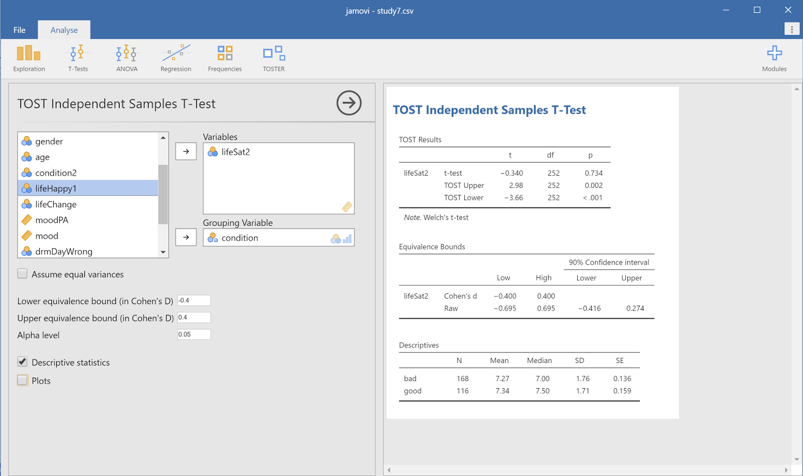
In the screenshot above you see the analysis and the results. By default, TOSTER uses Welch’s t-test, which is preferable over Student’s t-test (as we explain in this recent article), but if you want to reproduce the results in the original article, you can check the 
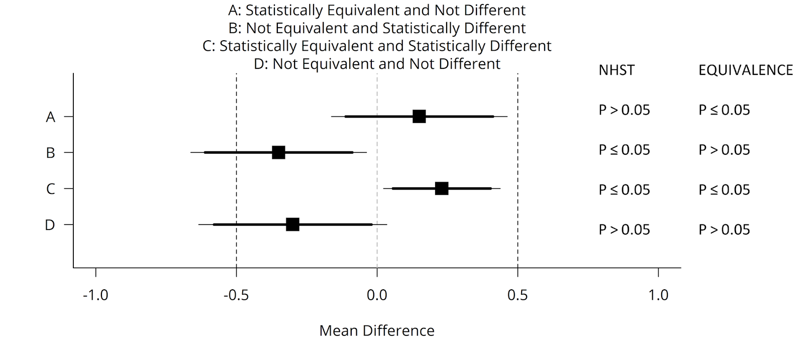
‘Assume equal variances’ checkbox. To conclude equivalence in a two-sided test, we need to be able to reject both equivalence bounds, and with p-values of 0.002 and < 0.001, we do. Thus, we can reject an effect larger than d = 0.4 or smaller than d = -0.4, and given these equivalence bounds, conclude the effect is too small to be considered support for the presence of an effect that is large enough, for our current purposes, to matter.

Jamovi runs on R, and it’s a great way to start to explore R itself, because you can easily reproduce the analysis we just did in R. To use equivalence tests with R, we can download the original datafile (R will have no problems with NA as missing values), and read it into R.  Then, in the top right corner of jamovi, click the … options window, and check the box ‘syntax mode’.


You’ll see the output window changing to the input and output style of R. You can simply right-click the syntax on the top, right-click, choose Syntax>Copy and then co to R, and paste the syntax in R:


Running this code gives you exactly the same results as jamovi.

I collaborated a lot with Jonathon Love on getting the TOSTER package ready for jamovi. The team is incredibly helpful, so if you have a nice statistics package that you want to make available to a huge ‘not-yet-R-using’ community, I would totally recommend checking out the developers hub and getting started! We are seeing all sorts of cool power-analyses Shiny apps, meta-analysis spreadsheets, and meta-science tools like p-checker that now live on websites all over the internet, but that could all find a good home in jamovi. If you already have the R code, all you need to do is make it available as a module!

If you use it, you can cite it as: Lakens, D. (in press). Equivalence tests: A practical primer for t-tests, correlations, and meta-analyses. Social Psychological and Personality Science. DOI: 10.1177/1948550617697177

Friday, March 10, 2017

No, the p-values are not to blame: Part 53

In the latest exuberant celebration of how Bayes Factors will save science, Ravenzwaaij and Ioannidis write: “our study offers through simulations yet another demonstration of the unfortunate effect of p-values on statistical inferences.” Uh oh – what have these evil p-values been up to this time?

Because the Food and Drug Administration thinks two significant studies are a good threshold before they'll allow you to put stuff in your mouth, in a simple simulation, Ravenzwaaij and Ioannidis look at what Bayes factors have to say when researchers find exactly two p < 0.05.

If you find two effects in 2 studies, and there is a true effect of d = 0.5, the data is super-duper convincing. The blue bars below indicate Bayes Factors > 20, the tiny green parts are BF > 3 but < 20 (still fine).


 Even when you study a small effect with d = 0.2, after observing two significant results in two studies, everything is hunky-dory.


So p-values work like a charm, and there is no problem. THE END.

What's that you say? This simple message does not fit your agenda? And it's unlikely to get published? Oh dear! Let's see what we can do!

Let's define 'support for the null-hypothesis' as a BF < 1. After all, just as a 49.999% rate of heads in a coin flip is support for a coin biased towards tails, any BF < 1 is stronger support for the null, than for the alternative. Yes, normally researchers consider 1/3 > BF < 3 as 'inconclusive' but let's ignore that for now.

The problem is we don't even have BF < 1 in our simulations so far. So let's think of something else. Let's introduce our good old friend lack of power!

Now we simulate a bunch of studies, until we find exactly 2 significant results. Let's say we do 20 studies where the true effect is d = 0.2, and only find an effect in 2 studies. We have 15% power (because we do a tiny study examining a tiny effect). This also means that the effect size estimates in the 18 other studies have to be small enough not to be significant. Then, we calculate Bayes Factors "for the combined data from the total number of trials conducted." Now what do we find?


Look! Black stuff! That's bad. The 'statistical evidence actually favors the null hypothesis', at least based on a BF < 1 cut-off. If we include the possibility of 'inconclusive evidence' (applying the widely used 1/3 > BF < 3 thresholds), we see that actually, when you find only 2 out of 20 significant studies when you have 15% power, the overall data is sometimes inconclusive (but not support for H0).

That's not surprising. When we have 20 people per cell, and d = 0.2, when we combine all the data to calculate the Bayes factor (so we have N = 400 per cell) the data is inconclusive sometimes. After all, we only have 88% power! That's not bad, but the data you collect will sometimes still be inconclusive!

Let's see if we can make it even worse, by introducing our other friend, publication bias. They show another example of when p-values lead to bad inferences, namely when there is no effect, we do 20 studies, and find 2 significant results (which are Type 1 errors).


Wowzerds, what a darkness! Aren't you surprised? No, I didn't think so.

To conclude: Inconclusive results happen. In small samples and small effects, there is huge variability in the data. This is not only true for p-values, but it is just as true of Bayes Factors (see my post on Dance of the Bayes Factors here).

I can understand the authors might be disappointed by the lack of enthusiasm of the FDA (which cares greatly about controlling error rates, given that they deal with life and death) to embrace Bayes Factors. But the problems the authors simulate are not going to be fixed by replacing p-values by Bayes Factors. It's not that "Use of p-values may lead to paradoxical and spurious decision-making regarding the use of new medications." Publication bias and lack of power lead to spurious decision making - regardless of the statistic you throw at the data.

I'm gonna bet that a little less Bayesian propaganda, a little less p-value bashing for no good reason, and a little more acknowledgement of the universal problems of publication bias and too small sample sizes for any statistical inference we try to make, is what will really improve science in the long run.


P.S. The authors shared their simulation script with the publication, which was extremely helpful in understanding what they actually did, and which allowed me to make the figure above which includes an 'inconclusive' category (in which I also used a slightly more realistic prior when you expect small effects -I don't think it matters but I'm too impatient to redo the simulation with the same prior and only different cut-offs).

Monday, March 6, 2017

How p-values solve 50% of the problems with p-values


Greenland and colleagues (Greenland et al., 2016) published a list with 25 common misinterpretations of statistical concepts such as power, confidence intervals, and, in points 1-10, p-values. Here I’ll explain how 50% of these problems are resolved by using equivalence tests in addition to null-hypothesis significance tests.

First, let’s look through the 5 points we will resolve:

4. A nonsignificant test result (P > 0.05) means that the test hypothesis [NOTE DL: This is typically the null-hypothesis] is true or should be accepted.
5. A large P value is evidence in favor of the test hypothesis.
6. A null-hypothesis P value greater than 0.05 means that no effect was observed, or that absence of an effect was shown or demonstrated.
7. Statistical significance indicates a scientifically or substantively important relation has been detected.
8. Lack of statistical significance indicates that the effect size is small.

With an equivalence test, we specify which effect is scientifically or substantially important. We call this the ‘smallest effect size of interest’. If we find an effect that is surprisingly small, assuming any effect we would care about exists, we can conclude practical equivalence (and we’d not be wrong more than 5% of the time).

Let’s take a look at the figure below (adapted from Lakens, 2017). A mean difference of Cohen’s d 0.5 (either positive or negative) is specified as a smallest effect size of interest. Data is collected, and one of four possible outcomes is observed. 


Equivalence tests fix point 4 above, because a non-significant result no longer automatically means we can accept the null hypothesis. We can accept the null if we find the pattern indicated by A: The p-value from NHST is > 0.05, and the p-value for the equivalence test is 0.05. However, if the p-value for the equivalence test is also > 0.05, the outcome matches pattern D, and we can not reject either hypothesis, and thus remain undecided. Equivalence tests similarly fix point 5: A large p-value is not evidence in favor of the test hypothesis. Ignoring that p-values don’t have an evidential interpretation to begin with, we can only conclude equivalence under pattern A, not under pattern D. Point 6 is just more of the same (empirical scientists inflate error rates, statisticians inflate lists criticizing p-values): We can only conclude there is absence of evidence under pattern A, but not under pattern D.

Point 7 is solved because by using equivalence tests, we can also observe pattern C: An effect is statistically significant, but also smaller than anything we care about, or equivalent to null. We can only conclude the effect is significant, and that the possibility that the effect is large enough to matter can not be rejected, under pattern B. Similarly, point 8 is solved because we can only conclude an effect is non-significant and small under pattern A, but not under pattern D. When there is no significant difference (P > 0.05), but also no statistical equivalence (P > 0.05), it is still possible there is an effect large enough to be interesting.

We see p-values (from equivalence tests) solve 50% of the misinterpretations of p-values (from NHST). They also allow you to publish effects that are statistically significant because they reject the presence of a meaningful effect. They are just as easy to calculate and report as a t-test. Read my practical primer if you want to get started.

P.S. In case you are wondering about the other 50% of the misinterpretations: These are all solved by remembering one simple thing. P-values tell you nothing about the probability a hypothesis is true (neither about the alternative hypothesis, nor about the null hypothesis). This fixed points 1, 2, 3, 9, and 10 below by Greenland and colleagues. So if we use equivalence tests together will null-hypothesis significance tests, and remember p-values do not tell us anything about the probability a hypothesis is true, you’re good.

1. The P value is the probability that the test hypothesis is true; for example, if a test of the null hypothesis gave P = 0.01, the null hypothesis has only a 1 % chance of being true; if instead it gave P = 0.40, the null hypothesis has a 40 % chance of being true.
2. The P value for the null hypothesis is the probability that chance alone produced the observed association; for example, if the P value for the null hypothesis is 0.08, there is an 8 % probability that chance alone produced the association.
3. A significant test result (P 0.05) means that the test hypothesis is false or should be rejected.
9. The P value is the chance of our data occurring if the test hypothesis is true; for example, P = 0.05 means that the observed association would occur only 5 % of the time under the test hypothesis.
10. If you reject the test hypothesis because P 0.05, the chance you are in error (the chance your
‘‘significant finding’’ is a false positive) is 5 %.

References

Greenland, S., Senn, S. J., Rothman, K. J., Carlin, J. B., Poole, C., Goodman, S. N., & Altman, D. G. (2016). Statistical tests, P values, confidence intervals, and power: a guide to misinterpretations. European Journal of Epidemiology, 31(4), 337–350. https://doi.org/10.1007/s10654-016-0149-3
Lakens, D. (2017). Equivalence tests: A practical primer for t-tests, correlations, and meta-analyses. Social Psychological and Personality Science.